Video Anomaly Detection
Tackling the problem of automatically detecting unusual activity in video sequences
MERL Researcher: Michael Jones (Computer Vision).
Joint work with: Bharathkumar Ramachandra (North Carolina State University), Ashish Singh (University of Massachusetts-Amherst), Erik Learned-Miller (University of Massachusetts-Amherst).
Search MERL publications by keyword: Computer Vision, anomaly detection, video analysis, action detection
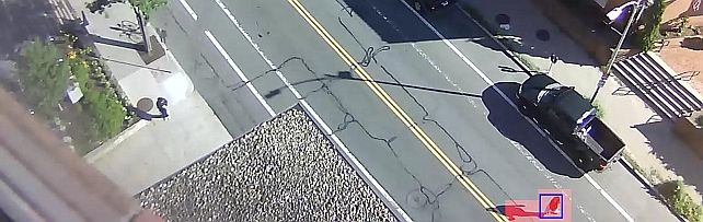
This research tackles the problem of automatically detecting unusual activity in video sequences. To solve the problem, an algorithm is first given video sequences from a fixed camera showing normal activity. A model representing normal activity is created and used to evaluate new video sequences from the same fixed camera. Any parts of the testing video that do not match the model formed from normal video are considered anomalous.
 found by our algorithm (a jaywalker). The blue square represents the ground truth labeled anomaly.")
Explainable Video Anomaly Localization
(This work originally appeared at CVPR 2023: Singh, A., Jones, M.J., Learned-Miller, E. Explainable Video Anomaly Localization, IEEE International Conference on Computer Vision and Pattern Recognition (CVPR), June 2023.)
Our solution to the problem of video anomaly detection consists of 3 stages: 1) training high-level attribute networks, 2) learning a model of a scene\'s normal activity, 3) anomaly detection.
Stage 1 is only done once and then used to provide high-level features for the latter two stages. Stages 2 and 3 are done for every new scene in which one wants to detect anomalies.
Stage 1: Training High-Level Attribute Networks
Deep networks are trained to estimate various high-level appearance and motion attributes of a video volume. A video volume is a fixed-size H x W x T volume of a video sequence where H is the height of a patch in a frame, W is the width and T is the number of frames.
The appearance attribute used in this work is the object class. We train a modified ResNext-50 architecture for our object recognizer using training images from CIFAR-10, CIFAR-100, MIO-TCD, as well as examples taken from surveillance video that we collected. We train on 8 different object classes (person, car, cyclist, dog, tree, house skyscraper, bridge) and use the penultimate 128-length layer of the network as a high-level feature vector that encodes the appearance of an image patch. To get a single feature vector representing a multi-frame video volume, we average the feature vectors computed separately for each frame.
We train 3 different motion attribute networks to represent the motion present in a video volume. These motion attributes are: a histogram of flow, a vector of motion speeds in each direction, and the fraction of stationary pixels in the video volume which is inversely proportional to the size of moving objects. The histogram of flow is represented using 12 bins (for every 30 degrees of motion direction) where each bin represents the fraction of pixels that are moving in a particular direction. The vector of motion speeds represents the average speed in pixels per frame for pixels moving in each of the 12 directions. The fraction of stationary pixels is the fraction of pixels in the video volume whose motion magnitude is below a small threshold. We train separate 3D convolutional networks to estimate each of these motion attributes directly from the RGB video volumes. The feature vectors output by the penultimate layers of each network is used as the high-level feature representing each type of motion attribute. High-level features are mapped to high-level attributes using the final linear layer of the respective neural network.

Once these appearance and motion attribute networks have been trained on outside data, they are used to provide high-level motion attributes and feature vectors that represent the types of objects and their directions and speeds of motion which are present in any scene. In other words, this stage is only done once and is not fine-tuned for each new scene. This makes our method much more practical for real-world usage and differentiates it from other approaches. These attributes were chosen because they are human-understandable. This allows the models that are learned for a scene to be human-understandable which in turn allows our system to provide intuitive explanations for its decisions about whether a piece of test video is anomalous or not.
Stage 2: Learning a Model of a Scene\'s Normal Activity
The next stage of our method is to build a model of a scene given nominal video of the scene. We first divide each frame into a set of overlapping spatial regions and scan a video volume of size H x W x T temporally over each nominal video. In our experiments, we choose H to be roughly the height of a person in the frame, W to be equal to H, and T to be 10 frames. We will learn a different model for each spatial region because anomalies are location dependent. What is normal in one region of a scene may be anomalous in another (for example, a person walking on a sidewalk may be normal while a person walking on a fence may be anomalous).
For each video volume in the nominal video, high-level feature vectors are extracted by evaluating each of the attribute networks on the video volume. The four feature vectors for a video volume are concatenated into one large feature vector. An exemplar selection algorithm is then run on all large feature vectors for a single spatial region (but many temporal positions). This results in a small set of feature vectors that span the entire set of feature vectors seen in the spatial region. Each feature vector in this small set is called an exemplar. The exemplar selection algorithm used in this work is very simple. We loop over all feature vectors and add each one to the exemplar set that has distance greater than a threshold from the nearest one already in the exemplar set. In other words, if a feature vector is already close to an exemplar, then it is not added to the set. The distance function we use is a sum of normalized Euclidean distances for each of the four types of feature vector.
The final model is a set of exemplars for each of the spatial regions in a video frame. The feature vectors that make up an exemplar can be mapped to high-level attributes which give our model its explainability.

Stage 3: Anomaly Detection
The final stage of our method is to detect, both spatially and temporally, any anomalies in test video of the scene. This is done by dividing the test video into video volumes in the same way as was done for building a model from nominal video. For each test video volume, a concatenated feature vector is computed by applying each of the four appearance and motion attribute networks. This feature vector is compared to the exemplars in the model for the corresponding spatial region. The distance to the closest exemplar is the anomaly score. If the anomaly score is above a threshold then the video volume is classified as anomalous.

Results
We tested our method on 5 publicly available test sets: UCSD Ped1, UCSD Ped2, CUHK Avenue, ShanghaiTech and Street Scene. The results are shown in the tables below. RBDC stands for Region-Based Detection Criterion, TBDC is Track-Based Detection Criterion and Frame is frame-level criterion. Numbers in red represent the best result for a given criterion and bold numbers are second best.

Table 1 shows the effect of varying the exemplar selection threshold on RBDC and TBDC accuracy as well as the total number of exemplars selected (NUM). Smaller NUM values mean a smaller, more efficient model, but allowing too few exemplars eventually negatively impacts accuracy. We chose a threshold of 1.5 in subsequent experiments since it yields good accuracy with a modest sized model.


Explainability
A big advantage of our EVAL method is that it can provide human-understandable explanations for its decisions. To visualize how our method can provide explanations, we first present an instrument panel for visualizing the high-level attributes computed for a video volume, shown in Figure 5. The instrument panel shows the object class estimates in the bar graphs at the top left, the fraction of stationary pixels in the bar graph at the top right, the histogram of flow in the circle at the bottom left, and the vector of speeds for each direction in the circle at the bottom right.
Now, consider the frame below taken from the Street Scene dataset. It contains a jaywalking anomaly shown in the red box.

We can first visualize the top ten exemplars learned for this spatial region:

The model has learned that this region typically contains cars either not moving or moving down and right relatively fast, or it contains unknown object that is not moving (i.e. stationary background). Occasionally, a part of a car will be captured and classified as an unknown object moving down and right fast.
If we visualize the feature vector estimated for a video volume containing the person jaywalking in the image above, we see that it is estimated as a person moving mainly right at moderate speed:

The closest exemplar to this test feature vector is:

This exemplar indicates an unknown object (most likely a car) moving down and right at a fast speed. The distance between the test feature vector and the closes exemplar is high and is therefore detected as an anomaly. By comparing the high-level attributes for the test feature vector and the closest exemplar, our method can say that the reason for the anomaly is that the test video volume contains an unexpected object class (person), moving in an unusual direction at an unusual speed.
Baseline Algorithms for Video Anomaly Detection
(This work originally appeared at WACV 2020: Ramachandra, B., Jones, M.J., "Street Scene: A new dataset and evaluation protocol for video anomaly detection", IEEE Winter Conference on Applications of Computer Vision (WACV), DOI: 10.1109/WACV45572.2020.9093457, February 2020, pp. 2569-2578.)
We describe two variations of a novel algorithm for video anomaly detection which we evaluate along with two previously published algorithms on the Street Scene dataset (described later).
The new algorithm is very straightforward and is based on dividing the video into spatio-temporal regions which we call video patches, storing a set of exemplars to represent the variety of video patches occurring in each region, and then using the distance from a testing video patch to the nearest neighbor exemplar as the anomaly score.
Algorithm Details
First, each video is divided into a grid of spatio-temporal regions of size H x W x T pixels with spatial step size s and temporal step size 1 frame. In the experiments we choose H=40 pixels, W=40 pixels, T=4 or 7 frames, and s = 20 pixels. See Figure 5 for an illustration. In this work, these spatio-temporal regions are called video patches while the previously described work called them video volumes.

The baseline algorithm has two phases: a training or model-building phase and a testing or anomaly detection phase. In the model-building phase, the training (normal) videos are used to find a set of video patches (represented by feature vectors described later) for each spatial region that represent the variety of activity in that spatial region. We call these representative video patches, exemplars. In the anomaly detection phase, the testing video is split into the same regions used during training and for each testing video patch, the nearest exemplar from its spatial region is found. The distance to the nearest exemplar serves as the anomaly score.
The only differences between the two variations are the feature vector used to represent each video patch and the distance function used to compare two feature vectors.
The foreground (FG) mask variation uses blurred FG masks for each frame in a video patch as a feature vector. The FG masks are computed using a background (BG) model that is updated as the video is processed (see Figure 6). The BG model used in the experiments is a very simple mean color value per pixel.
 and c) show two video patches consisting of 7 frames cropped around a spatial region. b) and d) show the corresponding blurred FG masks.")
The flow-based variation uses optical flow fields computed between consecutive frames in place of FG masks. The flow fields within the region of each video patch frame are concatenated and then vectorized to yield a feature vector twice the length of the feature vector from the FG mask baseline (due to the dx and dy components of the flow field). In our experiments we use the optical flow algorithm of Kroeger et al. (ECCV 2016) to compute flow fields.
In the model building phase, a distinct set of exemplars is selected to represent normal activity in each spatial region. Our exemplar selection method is straightforward. For a particular spatial region, the exemplar set is initialized to the empty set. We slide a spatial-temporal window (with step size equal to one frame) along the temporal dimension of each training video to give a series of video patches which we represent by either a FG-mask based feature vector or a flow-based feature vector depending on the algorithm variation as described above. For each video patch, we compare it to the current set of exemplars for that spatial region. If the distance to the nearest exemplar is less than a threshold then we discard that video patch. Otherwise we add it to the set of exemplars.
The distance function used to compare two exemplars depends on the feature vector. For blurred FG mask feature vectors, we use L2 distance. For flow-field feature vectors we use normalized L1 distance.
Given a model of normal video which consists of a different set of exemplars for each spatial region of the video, the anomaly detection is simply a series of nearest neighbor lookups. For each spatial region in a sequence of T frames of a testing video, compute the feature vector representing the video patch and then find the nearest neighbor in that region\'s exemplar set. The distance to the closest exemplar is the anomaly score for that video patch.
This yields an anomaly score per overlapping video patch. These are used to create a per-pixel anomaly score matrix for each frame.
More details of our algorithm can be found in our paper cited below.
New Dataset: Street Scene
In order to evaluate our video anomaly detection algorithm, we have created a new dataset containing video of a street scene in Cambridge, MA.
The Street Scene dataset consists of 46 training video sequences and 35 testing video sequences taken from a static USB camera looking down on a scene of a two-lane street with bike lanes and pedestrian sidewalks. See Figure 1 for a typical frame from the dataset. Videos were collected from the camera at various times during two consecutive summers. All of the videos were taken during the daytime. The dataset is challenging because of the variety of activity taking place such as cars driving, turning, stopping and parking; pedestrians walking, jogging and pushing strollers; and bikers riding in bike lanes. In addition, the videos contain changing shadows, and moving background such as a flag and trees blowing in the wind.
There are a total of 203,257 color video frames (56,847 for training and 146,410 for testing) each of size 1280 x 720 pixels. The frames were extracted from the original videos at 15 frames per second.
The 35 testing sequences have a total of 205 anomalous events consisting of 17 different anomaly types. A complete list of anomaly types and the number of each in the test set can be found in our paper.
Ground truth annotations are provided for each testing video in the form of bounding boxes around each anomalous event in each frame. Each bounding box is also labeled with a track number, meaning each anomalous event is labeled as a track of bounding boxes. Track lengths vary from tens of frames to 5200 which is the length of the longest testing sequence. A single frame can have more than one anomaly labeled.

Figures 7 and 8 show ROC curves for our baseline methods as well as a dictionary-based method (C. Lu, J. Shi and J. Jia, "Abnormal event detection at 150 fps in Matlab", ICCV 2013) and an auto-encoder method (M. Hasan, J. Choi, J. Neumann, A. Roy-Chowdhury, and L. Davis, "Learning temporal regularity in video sequences", CVPR 2016) on Street Scene using the newly proposed track-based and region-based criteria. The numbers in parentheses for each method in the figure legends are the areas under the curve for false positive rates from 0 to 1. Clearly, the dictionary and auto-encoder methods perform poorly on Street Scene. Our baseline methods do much better although there is still much room for improvement.

This dataset can be freely downloaded for research purposes from:
Region and Track-based Ground Truth files for other datasets:
We have created ground truth annotation files for the UCSD Ped1 and Ped2 datasets as well as CUHK Avenue dataset that can be used with the region-based and track-based evaluation criteria proposed in the Street Scene paper. Links to the zip file contain ground truth files for all 3 datasets can be found here:
ftp.merl.com/pub/streetscene/Ped1Ped2Avenue/Ped1Ped2Avenue_GTannotations.tgz
If you use or refer to this dataset, please cite the paper by Ramachandra and Jones titled, "Street Scene: A new dataset and evaluation protocol for video anomaly detection".
Software & Data Downloads
MERL Publications
- , "Street Scene: A new dataset and evaluation protocol for video anomaly detection", IEEE Winter Conference on Applications of Computer Vision (WACV), DOI: 10.1109/WACV45572.2020.9093457, February 2020, pp. 2569-2578.BibTeX TR2020-017 PDF Data
- @inproceedings{Jones2020feb2,
- author = {Ramachandra, Bharathkumar and Jones, Michael J.},
- title = {{Street Scene: A new dataset and evaluation protocol for video anomaly detection}},
- booktitle = {IEEE Winter Conference on Applications of Computer Vision (WACV)},
- year = 2020,
- pages = {2569--2578},
- month = feb,
- doi = {10.1109/WACV45572.2020.9093457},
- url = {https://www.merl.com/publications/TR2020-017}
- }
- , "Learning a distance function with a Siamese network to localize anomalies in videos", IEEE Winter Conference on Applications of Computer Vision (WACV), DOI: 10.1109/WACV45572.2020.9093417, February 2020, pp. 2598-2607.BibTeX TR2020-015 PDF
- @inproceedings{Jones2020feb,
- author = {Ramachandra, Bharathkumar and Jones, Michael J. and Vatsavai, Ranga},
- title = {{Learning a distance function with a Siamese network to localize anomalies in videos}},
- booktitle = {IEEE Winter Conference on Applications of Computer Vision (WACV)},
- year = 2020,
- pages = {2598--2607},
- month = feb,
- doi = {10.1109/WACV45572.2020.9093417},
- url = {https://www.merl.com/publications/TR2020-015}
- }
- , "A Survey of Single-Scene Video Anomaly Detection", IEEE Transactions on Pattern Analysis and Machine Intelligence, DOI: 10.1109/TPAMI.2020.3040591, Vol. 44, No. 5, pp. 2293-2312, November 2020.BibTeX TR2021-029 PDF
- @article{Jones2020nov,
- author = {Jones, Michael J. and Ramachandra, Bharathkumar and Vatsavai, Ranga},
- title = {{A Survey of Single-Scene Video Anomaly Detection}},
- journal = {IEEE Transactions on Pattern Analysis and Machine Intelligence},
- year = 2020,
- volume = 44,
- number = 5,
- pages = {2293--2312},
- month = nov,
- doi = {10.1109/TPAMI.2020.3040591},
- url = {https://www.merl.com/publications/TR2021-029}
- }
- , "Perceptual Metric Learning for Video Anomaly Detection", Machine Vision and Applications, DOI: 0.1007/s00138-021-01187-5, Vol. 32, No. 63, pp. 1-18, March 2021.BibTeX TR2021-028 PDF
- @article{Ramachandra2021mar,
- author = {Ramachandra, Bharathkumar and Jones, Michael J. and Vatsavai, Ranga},
- title = {{Perceptual Metric Learning for Video Anomaly Detection}},
- journal = {Machine Vision and Applications},
- year = 2021,
- volume = 32,
- number = 63,
- pages = {1--18},
- month = mar,
- doi = {0.1007/s00138-021-01187-5},
- url = {https://www.merl.com/publications/TR2021-028}
- }